Optimal integration weights in qubit readout
Introduction
The state of a superconducting qubit can be measured using a probe microwave signal. By analyzing the probe after it has interacted with the system, we extract its phase and amplitude values (or, equivalently, the signal quadratures) and assign the qubit state either to 0 or 1.
But how to extract the quadrature values of a pulse, and how to do so in an optimal, noise-resistant way?
The objective of this post is to go through the math and the code for finding the optimal integration weights of a readout. These are functions that weigh each data point of a readout integration process, assigning high weight to time bins that carry high information content of the qubit and assigning low weight to instants in which noise dominates. I will show the relevant Python code and you will be able to apply this procedure regardless of the control electronics that are used.
Table of Contents
- Introduction
- Table of Contents
- The Is and Qs of a signal
- Calculating optimal integration weights
- Conclusion
The Is and Qs of a signal
This is what the ADC-acquired signal looks like:
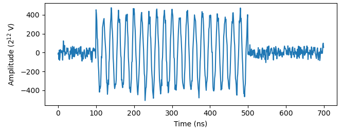
In this example, the digital signal $s[n]$ has a carrier frequency $\omega_{IF} =$50 MHz and a simple 400ns square envelope. In my case, the ADC has a resolution of $2^{-12}$, so the amplitude of the acquired pulse trace can be converted to volts by multiplying by the same factor.
Let’s see how to calculate the pulse quadratures. Besides the signal, the ADC also acquires white noise that travels through the lines. To parse the readout information from the noise, we project the pulse onto a constant wave $K[n]$ oscillating at the same frequency:
\[K[n] = e^{i\omega_{IF} t_s n}\] \[\rightarrow X[\omega_{IF}] = \braket {K|s} = \sum_{n=0}^Ns[n]e^{-i\omega_{IF} t_s n} = I +iQ.\]The projection $X[\omega_{IF}]$ is equivalent to the Fourier transform of the signal at frequency $\omega_{IF}$. We are thus ignoring all other frequency components. Since $X[\omega_{IF}]$ is a complex number, it can be written as a sum of a real part $I$ to an imaginary part $Q$. These are the quadratures of $s[n]$.
The quadratures are obtained as a sum, or integration, of the signal multiplied by a demodulation factor:
\[I = 2^{-12}\sum_{n=0}^Na[n]\cos(\omega_{IF}t_sn),\] \[Q = -2^{-12}\sum_{n=0}^Na[n]\sin(\omega_{IF}t_sn).\]We can generalize the quadrature integration formula as a function of weight functions $w_s[n]$ and $w_c[n]$:
\[d = 2^{-12}\sum^N_{n=0}a[n]\left(w_c\left[n\right]\cos(\omega_{IF}t_s n + \phi) +w_s\left[n \right]\sin(\omega_{IF}t_s n + \phi)\right).\]For $I$ integration, $w_c[n] = 1$ and $w_c[n]=0$, while the oppposite is true for $Q$.
A prototypical qubit readout can simply use $I$, $Q$, or functions such as $\sqrt{I^2 + Q^2}$. Exciting the qubit will change the quadratures of the acquired signal and will show up as a feature in the experiment. But we want to go further. By optimizing the integration weights, we can reduce the impact of noise in the integration. We can also project the information into a single quadrature, say $I$, to be used for optimal readout. So let’s see what else integration weights can offer.
Rotating the signal in phase space
As previously mentioned, $X[\omega_{IF}]$ is a complex number. A rotation in phase space is as simple as a multiplication by a phase factor:
\[X[\omega_{IF}] = I+iQ = (I'+iQ')e^{-i\delta} = X'[\omega_{IF}]e^{-i\delta}.\]The quadratures are transformed as
\[\begin{pmatrix} I'\\Q'\end{pmatrix} = \begin{pmatrix} \cos \delta && -\sin\delta\\ \sin\delta &&\cos \delta\end{pmatrix} \begin{pmatrix} I\\Q\end{pmatrix},\]which can be rewritten directly as quadrature integration:
\[I' = 2^{-12}\sum_{n=0}^Na[n]\left(\cos{\delta}\cos(\omega_{IF}t_sn) + \sin\delta\sin(\omega_{IF}t_sn) \right)\] \[Q' = 2^{-12}\sum_{n=0}^Na[n]\left(\sin{\delta}\cos(\omega_{IF}t_sn) - \cos\delta\sin(\omega_{IF}t_sn) \right)\]So the rotated quadratures have the same general structure as the original quadratures, except for a different choice of integration weights. The rotation angle is determined by the $\arctan(w_s/w_c)$, or, equivalently, by the argument of the complex number $w_c + iw_s$. We will employ this knowledge in the next section.
Calculating optimal integration weights
As mentioned beforehand, the objectives of optimizing integration weights are two:
- Increase the weights when the information carried by the signal is high compared to the noise; decrease weights otherwise,
- Rotate the signal in phase space so the information is encoded on a single quadrature.
How to know which sections of the signal carry more or less information about the qubit? It is not too complicated. The signal goes through a trajectory in phase space as a function of time, and the path changes whether the qubit is in $\ket{0}$ or $\ket{1}$.
To get the trajectory of the signal, we first calculate its complex envelope. The envelope (figure on the left) is essentially the downconversion of the signal by the frequency $\omega_{IF}$, and is also a sequence of complex numbers that describe the path in phase space (figure on the right).
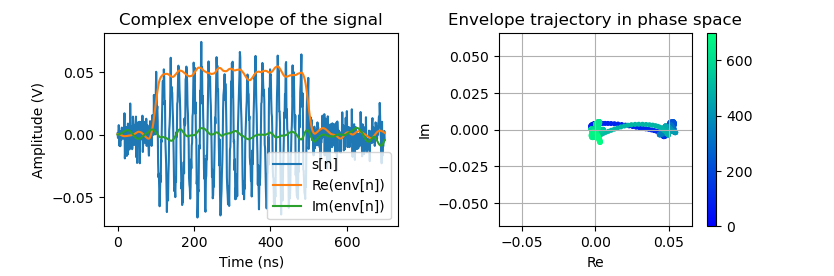
In the next section, we go through the calculation step-by-step.
Obtaining the signal envelopes
Consider first the simple time-continuous case where $a(t) = A\cos(\omega t+ \phi)$. We know $\omega$ and we want to obtain $A$ and $\phi$. This can be done by multiplying the trace by an exponential factor $e^{j\omega t}$:
\[\begin{align*} a(t)e^{j\omega t} &= A\cos(\omega t)\cos(\omega t + \phi) + iA\sin(\omega t)\cos(\omega t + \phi) \\ &= \frac{A}{2}(\cos(\phi) + \cos(2\omega t +2\phi)) + i\frac{A}{2}(-\sin(\phi) + \sin(2\omega t +2\phi)) \end{align*}\]Now we have two frequency components, DC and $2\omega$. The cool thing is that now one of these components does not oscillate in time and carries both $A$ and $\phi.$ The uncool thing is that the $2\omega$ component must be filtered. After filtering, the signal is
\[\left(a(t)e^{i\omega t}\right)_{DC} = \frac{A}{2}e^{-i\phi},\]And the parameters $A$ and $\phi$ are obtained through simple calculation. Note the resulting signal has half the amplitude and the phase is flipped.
Back to the readout signal example, we will take the product
\[s_{rot}[n]= s[n]e^{i\omega_{IF}t_sn}\]And then apply a Hann filter by calculating the convolution
\[s_{filtered}[n]= (s_{rot}*h)[n] = \sum_{n'=0}^Ns_{rot}[n']h[n-n'],\]where $h[n]$ is the impulse response of a Hann filter, which acts as a low-pass filter to eliminate $2\omega_{IF}$ components on the signal. Since the phase is flipped and the amplitude is halved, we can get the envelope as
\[env(s) = \frac{1}{2}(s_{filtered}[n])^*.\]Important: We need to make sure the acquired signal $s[n]$ does not have a DC offset. It can be simply removed digitally by subtracting the signal average. Otherwise, the envelope will present ripples oscillating at frequency $\omega_{IF}$ corresponding to the upconverted DC offset.
Optimal integration weights as a difference in envelopes
Suppose two signals $s_g[n]$ and $s_e[n]$ are acquired when the qubit is in the ground and excited state. Their envelopes will have very distinct trajectories in phase space. The optimal integration weights, the function that extracts the maximum qubit state discrimination information from the signals, is the difference between the two complex envelopes:
\[w_{opt} = \textrm{env}(s_g)[n] - \textrm{env}(s_e)[n] = W[n]e^{i\theta[n]}.\]If the envelopes are equal at an instant $n_{eq}$, there is no information about the qubit state and $w_{opt}[n_{eq}] = 0$.
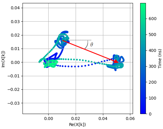
Additionally, the phase of $w_{opt}[n]$ will rotate the excited- and ground-state $(I,Q)$ pairs so they are aligned with the real axis of the complex plane, and therefore we only need to care about the quadrature $I$ during readout. See the picture below, which shows the two trajectories in phase space. The red arrow is a demonstration of $w_{opt}[n]$ at a given point in time. It has a phase of $arg(w_{opt}[n]) = -\theta[n]$, which we eliminate by rotating the plane by $\theta = arg(w_{opt}[n])$ during the demodulation.
Returning to the quadrature integration equation, we implement the weights by assigning
\[w_c = Re(w_{opt}) =W[n]\cos\theta[n]\] \[w_s = -Im(w_{opt}) = -W[n]\sin\theta[n]\]which gives the optimal quadrature $I_{opt}$ to be used in qubit readout.
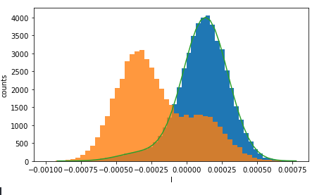
To show how the results look like in practice, I got a graph from a recent experiment I did. The blue histogram shows the frequency of values of $I_{opt}$ when the qubit is prepared in the ground state $\ket{0}$. Notice it has essentially a Gaussian shape with mean $I_{g}$. The orange histogram shows the same experiment, but when the qubit is prepared in the excited state $\ket{1}$. If we ignore the decay $\ket{1} \rightarrow \ket{0}$ that occurs during the measurement, it also has a Gaussian shape around a value $I_{e}$. Knowing these values is essential for single-shot readout: in a single measurement of $I_{opt}$, we can assign the state of the qubit according to whether it is closer to $I_{g}$ or $I_{e}$. The state discrimination problem is uni-dimensional, so it is convenient that we have projected it to a single quadrature.
Conclusion
Now you know how to read a qubit state by calculating the quadrature components of a probe signal. And also how to optimize this process by calculating the quadratures through weighted integration. The process involves some signal processing protocols, but hopefully these were well-justified. By following this recipe, you will also be able to implement single-shot readout of a superconducting qubit. 加油!