If you wish to learn more about circuit quantum electrodynamics (cQED), this is where you should start. To eventually understand the design of superconducting quantum processors, the best strategy is to first understand the simplest quantum circuit: the superconducting resonator.

This post will give the first introduction to this device. First, we take a look at resonators in classical physics. Then we lay down the recipe for translating classical circuits into quantum mechanics. We apply this procedure to a lump-element resonator, which is a simple but useful model. To wrap up, we will see how to deal with circuits with multiple resonant modes. By the end, you will have an idea of how to apply the same procedure to other circuits, as will be done in future posts.

Table of Contents

• Table of Contents
• The classical resonator
• Quantization of superconducting resonators
• Diagonalizing coupled resonators
  • Capacitive coupling
  • Hybridization of coupled resonant modes
• Conclusion

The classical resonator

In classical electrical circuits, the resonator is nothing more than an LC circuit. That is, it can be modeled as a capacitor shunted by an inductor. If one node of the circuit is grounded, the second node has a voltage $V$. Then the inductor follows the dynamical equations

Where $i$ is the current flowing through the inductor and the node flux is defined as $\phi = \int_{-\infty}^tV(t)dt$. $E_L$ is the inductive energy stored in the circuit at a given moment $t$, assuming all variables are null at $t\to-\infty$. The capacitor shares the current and voltage over the inductor and follows the known dynamics

$E_C$ is the capacitive energy stored in the circuit at a given moment. So far, no groundbreaking physics has been shown. This circuit behaves as a harmonic oscillator, as we see in the dynamical equation of the current:

The solution is $i(t) = i_0\cos(\omega_r t + \theta)$, where the current oscillates with a frequency $\omega_r = (LC)^{-\frac{1}{2}}$. This type of system has been studied to exhaustion by any physicist, so there’s no need to talk more about it. The interesting part comes next when this circuit becomes quantum.

Quantization of superconducting resonators

cQED is the formulation of circuits in the quantum mechanical regime. It is based on a very straightforward (although complex) premise that we can quantize the parameters of the circuit. The node charges $Q$ and fluxes $\phi$ become quantum variables described by operators and the circuit state evolves according to the Schrodinger equation. But to follow through with this idea, as with any quantum problem, we need to find the correct Hamiltonian.

The procedure to find a Hamiltonian is often done wrongly, so it is worth showing the general step-by-step. The first step is to obtain the classical Hamiltonian of the circuit, and then substitute the conjugate pairs of dynamical variables by non-commuting operators. In circuit QED, that is:

1. Numerate all the nodes of the circuit and define the variables $Q_k$ and $i_k$ for the $k$-th node.

In the case of the resonator, there is only one pair of $Q$ and $i = \dot{Q}$.

2. Write the Lagrangian in terms of these variables $L(Q_k, i_k, t) = T - V$. T and V are the kinetic and potential energies of the system, respectively.

The kinetic energy is the capacitive energy $T = E_C$, while the potential energy is the inductive energy $V = E_L$. Our lagrangian is

3. Calculate the generalized momentum $p_k$ of each charge $Q_k$: $p_k = \frac{\partial L}{\partial i_k}$

The generalized momentum is $p = -Li = \phi$!

4. Apply the Legendre transform to the Lagrangian to obtain the classical Hamiltonian: $H(Q_k, p_k, t) = L - \sum_k p_k i_k$

In this step, we have to remember to rewrite every $i_k$ in terms of its momentum. The solution is again very simple for the resonator:

The Hamiltonian is essentially the total energy $E_C + E_L$ in terms of $Q$ and $\phi$. It is common to jump to this step and simply write the Hamiltonian as the total energy, and it is correct most of the time. But this might not be so easy to do in more complicated systems, so I decided to show how to get here in the correct way.

5. Quantize the Hamiltonian by replacing the variables $Q_k$ and $\phi_k$ by operators $\hat{Q}_k$ and $\hat{\phi}_k$ such that $[\hat{Q}_k, \hat{\phi}_k] = i\hbar$

This step is sometimes called “first quantization”. It is a simple substitution that makes the function $H(Q, \phi)$ into an operator $\hat{H}(\hat{Q}, \hat{\phi})$. The Hamiltonian of a superconducting resonator then is:

As expected, this is the Hamiltonian of a quantum harmonic oscillator. We can rewrite the operators as functions of ladder operators:

so the Hamiltonian is rewritten as (dropping hats and the constant $1/2$ factor and setting $\hbar = 1$)

This is the typical form we treat resonators in circuit QED. Many other circuits will include an $a^{\dagger} a$ term in its Hamiltonian, and we frequently use this term to implicitly model the environment. Because it is so common, we need to know how to simplify systems in which two harmonic oscillator terms are coupled.

Diagonalizing coupled resonators

When two superconducting resonators are put geometrically close, their fields overlap. The electromagnetic field generated by current and charge accumulation in one resonator will induce current and charge in the other. That is called capacitive coupling and is how two superconducting circuits can interact with each other. Let’s start by deriving the capacitive coupling term to understand how it works.

Capacitive coupling

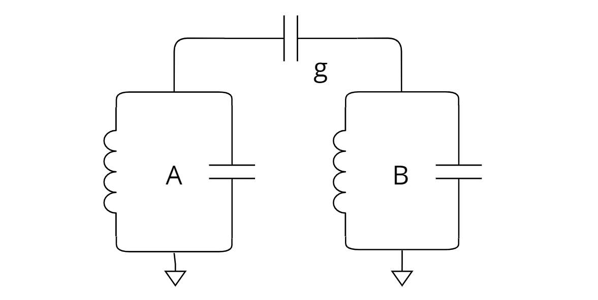
The circuit in the figure above shows two LC circuits A and B whose nodes are connected by a gate capacitance $C_g$. Let us define $V_A$, $V_B$ and $V_g$ as the voltages over each element, with orientations such that Kirchhoff voltage law reads as

In terms of flux, we have

Following the quantization procedure in the last section and substituting $\dot{\phi_g}$, the Lagrangian is

The conjugate momenta to $\phi_A$ and $\phi_B$ are, respectively:

These equations are not as trivial to find if not following the step-by-step quantization. Rewriting in terms of the first flux derivative:

where $D = C_AC_B + C_AC_g + C_BC_g$. Now we get the Hamiltonian in terms of $\phi_A$, $\phi_B$, Q$_A$ and Q$_B$:

$H_A$ and $H_B$ are each resonator’s term, while $H_g$ describes the coupling between them:

Finally, we quantize the canonical variables by substituting for operators $Q_i \rightarrow \hat{Q}_i$, $\phi \rightarrow \hat{\phi}_i$. We can further develop the Hamiltonian by defining ladder operators $\hat{a}$, $\hat{b}$ that diagonalize $H_A$ and $H_B$, leading to ($\hbar = 1$)

The capacitive coupling Hamiltonian is represented by a coupling factor $g$, which has the value

The capacitive coupling is a very important term in circuit QED. The interactions between circuits, and of these with external drives, are usually described by this Hamiltonian for a given factor $g$. It is then essential to understand how to deal with this term once it shows up. In the next section, I will show how we can redefine the ladder operators to hybridize the modes $\hat{a}$ and $\hat{b}$, making the coupling term vanish.

Before we proceed, I want to introduce a simplifying approximation that is also a very frequently used technique. Expanding the capacitive coupling term gives

There are two types of terms here: the co-rotating terms $a^{\dagger}b$, $ab^{\dagger}$, and the counter-rotating terms $a^{\dagger}b^{\dagger}$, $ab$. There are many ways to interpret these two types of terms, so I will offer one explanation. The co-rotating terms describe an evolution where one excitation is removed from one of the resonators while one excitation is created in the other resonator. The energy required to activate such dynamics is $\hbar (\omega_A - \omega_B) $, which is the difference in energy between the excitations. Meanwhile, the counter-rotating terms describe the simultaneous gain ($a^{\dagger}b^{\dagger}$) or loss ($ab$) of excitations from both resonators, implying a change of energy of magnitude $\hbar (\omega_A + \omega_B)$. As we work in a regime where $\omega_A \approx \omega_B$, the counter-rotating terms have a much higher “energy cost”. Unless $g$ has a relatively high value ($g \gtrsim \omega_A + \omega_B$), we can safely ignore them. This is called the rotating wave approximation (RWA) and it leaves only the co-rotating terms in the Hamiltonian:

Hybridization of coupled resonant modes

Let’s go back to our uncoupled (bare) resonator modes $\omega_A a^{\dagger}a$ and $\omega_B b^{\dagger}b$. As seen in the last section, they come from two separate LC circuits with resonance frequencies $\omega_{A, B}$. However, once they are connected by a gate capacitance $C_g$, the resonant modes are disturbed and $\omega_{A, B}$ stop being resonance frequencies of the system. We want to find the new resonant modes with frequencies $\tilde{\omega}_{A,B}$, and that turns out to always be possible through a mindful redefinition $\hat{a} \rightarrow \tilde{a}$, $\hat{b} \rightarrow \tilde{b}$.

Rewriting the Hamiltonian (after the RWA) in the matrix form:

Turns out the Hamiltonian is described by a symmetric matrix, that is, equal to its transpose. Symmetric matrices with non-degenerate eigenvalues always have orthogonal eigenvectors - this means they can be diagonalized just by frame rotation. So there exists a rotation angle $\Lambda$ such that

That is, in such a frame, there are two decoupled resonant modes with frequencies $\tilde{\omega}_{A,B}$. The ladder operators of the new resonant modes are calculated from the change of frame

so that the resonant new modes are hybridizations of the previous modes: e.g. $\tilde{a} = \cos\Lambda a + \sin\Lambda b$.

This procedure can be readily generalized to more than two resonators. In fact, the same technique is used to deal with the linear terms of nonlinear circuits such as qubits, simplifying qubit-resonator or qubit-qubit hamiltonians.

Conclusion

We have gone through the mathematical details of treating a resonator in circuit QED. We covered the quantization procedure from ground-up, through which the resonator reveals the dynamics of a quantum harmonic oscillator. Then, we saw how two resonators can be coupled together and how to simplify the Hamiltonian in such cases.

The resonator is too simple of a circuit, and we can’t do quantum computation by relying only on them. So, in the future, I will write about how we can model transmons in cQED and how we can use them to make qubits. The knowledge from this post will be essential, so try to develop the equations yourself. 加油!